Jason Thomas - I like to make stuff

August 11, 2021 @ 15:04

Using Gnu Octave inside Jupyter Notebook

latex, Octave and a chart, all together

Recently I have used Jupyter Notebook for using Octave and currently it's my favourite environment. This article will show how I've been using Octave with Jupyter Notebook.

This post:

offers some quick examples
explains why I avoid Matlab, if I am able
shows how to setup Jupyter Notebook to run Octave
offers some tips about how to make functions more useful
shows how to install the Symbolic package

I should make a disclaimer; I'm a maths student and former software developer and perhaps your needs are different to mine.

What is Octave

It's an open source and free alternative to Matlab. I do understand that Matlab has more packages available, but I only really do elementary linear algebra at the moment and have no need for all of Matlab's other stuff. I have no issues switching back to Matlab if a future employer needs me to.

Octave does offer packages like the Symbolic package (if you've ever typed syms x y ... in Matlab you'll know what this is).

What's wrong with Matlab (if you ask me)

There are three things:

It's a proprietary language. I'm not inclined to write code in my spare time to then put the work on Github or wherever else, to then lose my scripts if I lose access to Matlab.
I dislike the IDE. The Matlab IDE doesn't seem to allow me to use Vim keybindings. I couldn't find how to set this up.
It's not available as a CLI and you must run their GUI. This is annoying for me as I'd like the option to run scripts as executable files.

What's great about Jupyter Notebook

It supports Latex. I often like having functions written down this way before I implement the code. Sometimes I like to just have a combination of code and Latex to really highlight certain things
It provides immediate feedback. I like having a series of cells where I do individual steps. Imagine combining Matlab's code editor and command line panel into one, except that it's better looking
It supports Vim keybindings, which I have become pretty dependent on

The only downside I've found... and a workaround

A notebook can only embed static Octave plots inline. If you want to see an interactive plot/meshgrid etc, then in an Octave cell run %plot gnuplot. This will switch to using the pop-out window. To toggle this back, do %plot inline.

Some examples I've made recently

Example .m file with docstring. These help in Jupyter Notebook
Example notebook that has examples of Octave code, Latex cells and charts
Example notebook where I document what is essentially a script using snippets of Latex.

Installing Jupyter Notebook

These steps assume you use a Debian-like machine, like Ubuntu or Mint.

Everything after running Jupyter Notebook is the same.

Install octave

sudo apt update
sudo apt upgrade
sudo apt install octave

Install a Virtual Environment to localise your Python packages.
```
sudo apt install virtualenv
```

Create an env and activate it

virtualenv venv -p python3
source /venv/bin/activate

Install the dependencies

pip install sympy==1.4 jupyter octave-kernel

Note: If you want to install the Symbolic package in Octave, then at the moment, you must use that particular version of Sympy.

Run Jupyter
```
jupyter notebook
```
In a new notebook, select the Octave kernel

Writing Notebook-friendly functions

Jupyter Notebook will allow you to load functions from the path relative to your notebook.ipynb file.

It also allows you to display docstrings that will help you use the function while inside the notebook.

Here is a minimal docstring for the top of a function in Octave:

## -*- texinfo -*-
## @deftypefn FUNCTION_NAME(@var{PARAMETER_NAME_1})
## @deftypefnx FUNCTION_NAME(@var{PARAMETER_NAME_1}, @var{PARAMETER_NAME_2})
## SOME TEXT TO DESCRIBE ITS BEHAVIOUR 
## @end deftypefn

Where @deftypefn is the function's standard behaviour and @deftypefnx is the alternative use.

A docstring wants to go as a comment directly below the function declaration, and above the body.

In your running Notebook instance, type the function's name and then press SHIFT-TAB to see the function description.

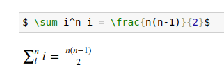
Using Latex

This is a good reason to use a Notebook. Create a new cell and then change its type to Markdown. Then $ LATEX HERE $ in between the $ symbols.

For example :

latex for Guass formula

Loading packages

One I mentioned earlier was the Symbolic package.

In a Jupyter Notebook cell, do: pkg install -forge symbolic

That's a once-off.

Then do pkg load symbolic and save that to your Notebook near the top.

Here's an example:

    syms x y z;

    poly_1 = x^2 + 3;
    poly_2 = x^3 - 3*x^2 -1;
    poly_3 = 4*x^3 - 8;

    addition_combined = poly_1 + poly_2 + poly_3;
    multiplication_combined = poly_1 * poly_2 * poly_3;
    multiplication_combined / diff(addition_combined)

OK, I hope this has helped, thanks for reading.